Machine Learning validates the AMO model

What ML does for modeling the ENSO, it also applies to the Atlantic Multidecadal Oscillation. And arguably it does it more impressively.

Apr 17, 2023

As a prerequisite, please read the previous Sub(Surface)Stack article on modeling the El Nino Southern Oscillation (ENSO), which is a follow-on to earlier published research.

SubSurface

Machine Learning validates the ENSO model

2 months ago · Puͣkiͧte̍

The applications of machine learning (ML) are exploding right now, so it’s a good time to check how a artificial neural network (NN) model would help resolve previous findings on the cause of AMO.

Premise

As the ENSO is to the Pacific Ocean, the Atlantic Multidecadal Oscillation (AMO) is to the Atlantic Ocean. One distinction is that the AMO is not strictly an equatorial phenomena, with measurements of sea-surface temperature anomalies extending into the north Atlantic. This gives a hint that the symmetric tidal forcing used for the ENSO model may have more of an asymmetric hemispherical bias for the AMO. Recall that for the ENSO model, alternating-sign semiannual delta impulses modulated a long-period tidal forcing f(t).

\(\int_{-\infty}^{\infty} \left(\sum_{n=0}^{\infty} (-1)^n \delta(t-nT)\right) f(t) dt \)

Now consider that the positive impulses have a different prefactor A, than the negative impulses B occurring 6 months later:

\(\int_{-\infty}^{\infty} \left(A \sum_{n=0}^{\infty} \delta(t-2nT) - B\sum_{n=0}^{\infty} \delta(t-(2n+1)T) \right) f(t) dt \)

Plotting both A an -B integrated series on the same chart illustrates a striking character indicative of a strong aliasing effect.

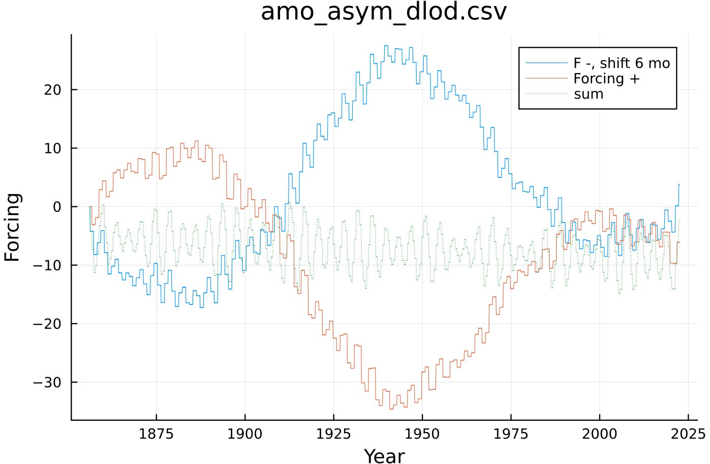
Note that the forcing goes through a strong multidecadal modulation hinting at the character of AMO itself. This is in strong contrast to the ~3.8 year cycle of the symmetric forcing (see dotted time-series in the above chart, showing the summed A-B, where |A|=|B|) which is applied to the ENSO model.

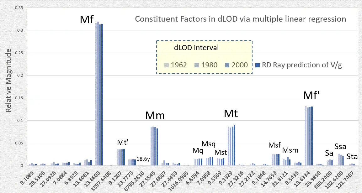
What causes this multidecadal modulation? With a little digging it can be traced to the long-term annual constructive interference of the Mt tidal factor (referenced on the LOD constituent chart shown in the previous article). Mt is a well-known factor resulting from nonlinear mixing of the Mf and Mm tides.

The impact of the Mt factor is due to the fact that an integer multiple of cycles almost exactly match the annual period. This means that small Mt forcings gradually accumulate year-to-year, unlike the other factors which largely cancel within a few years. The end result is that the complete constructive/destructive interference cycle is between 120 to 130 years depending on the precision of the Mt period.

As with the ENSO model’s symmetric forcing, this particular tidal forcing was previously isolated for the AMO model and worked well within the context of the LTE fluid dynamics formulation

. A modest LTE modulation was required and this then matched to the 60 to 65 year period of the AMO. The question is then whether a neural network could also effectively match the tidal factors with observations via training on select intervals.

Machine Learning

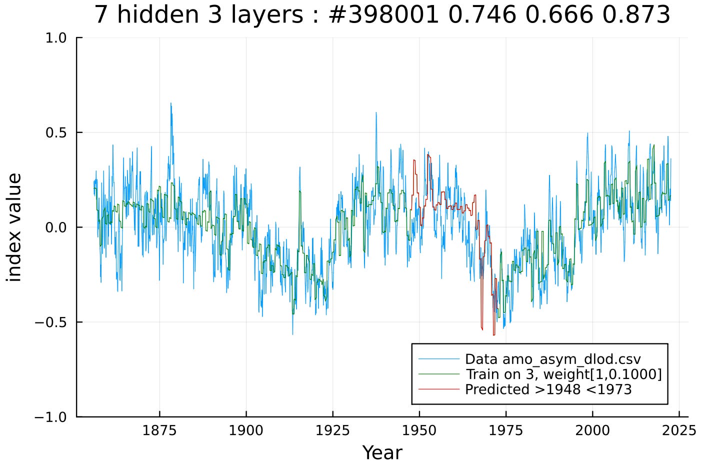
Intuition would anticipate that a nonlinear neural network would quickly find the frequency doubling interaction necessary to transform the intrinsic 120-130 year forcing cycle to the 60-65 year AMO cycle. To facilitate this, the two anti-symmetric tidal forcing time-series shown above were used as NN inputs (along with a lightly-weighted linear time ramp).

Sure enough, the Julia Flux NN configuration locked into this long AMO cycle almost immediately and then used most of the compute time reducing the loss function on the otherwise noisy-appearing training interval. The RED line is the prediction evaluation based on training of the enclosing outer discontinuous interval.

For a smaller NN chain on a different evaluation interval, the results are equally promising (though not at as fine a resolution).

Occasionally the NN will lock into a non-optimal fit but for the majority of training runs, it will follow the detailed time-series profile. The turn-around time is fast enough that trying different chain configurations is cheap and convenient. Through some trial-and-error, different training parameters were found to apply better to AMO in comparison to ENSO

This video shows the training in operation

(note: video also on Twitter

: https://twitter.com/WHUT/status/1646140396441935874 )

It’s not exactly clear how the NN is weighting the chain during training but a simple and straightforward candidate is to rectify each of the forcings to only positive values and then sum the result

. This would create to first-order a frequency doubled waveform that would align with the observed AMO. The finer more rapid fluctuations are modulated along with the gradual slower variations, which one can see from the video.

To try to understand the NN internal state, we scan the entire 2-D forcing space and watch how it traverses the output modulation over time, as shown in the video below. Note that the NN clearly sets up a modulation boundary along x = -y (with + and - width also indicated) which is essentially close to the input forcing envelope, observed by watching the moving dot.

(Twitter version: https://twitter.com/WHUT/status/1646704411052318720 )

The weighting of the layered NN chain is extracted from the following Julia extract, where m is the model. Would need to carefully reverse engineer this to find the actual weightings corresponding to the A and B coefficients and any non-linear interactions between the two.

for (i, layer) in enumerate(m.layers)
   if isa(layer, Dense)
      println("Layer $i weights:")
      println(layer.weight)
      println()
    end
end

Implications

In comparing the results of the AMO NN model against the ENSO NN model, it reinforces the significance of the geophysical explanation. Marcus asked “Does an Intrinsic Source Generate a Shared Low-Frequency Signature in Earth’s Climate and Rotation Rate?“

. The connection between AMO, climate variability on this scale, LOD variations, and the influence of tides on LOD forms a sort of jigsaw puzzle. Entirely consistent if not plausible that the Mt tide is amplifying the oceanic response, leading to long-term integrated fluidic weight redistributions with the conservation of angular momentum leading to concurrent LOD variations.

As a counter, some claim that the AMO is not even a naturally occurring oscillation

arguing that other factors such as volcanic activities and AGW itself could plausibly cause similar cyclic-appearing variations.

Perhaps the larger point of this article and the prior one is that future ML experiments on indices such as ENSO and AMO will certainly find these same patterns, but, alas, may not know how to interpret the results. Fortunately, the geophysics described here may help resolve the mystery.

p.s. The next SubSurfaceStack article is on ML of PDO, which serves as a transitional link between ENSO and AMO.

Pukite, P., Coyne, D., & Challou, D. (2018). Mathematical geoenergy: discovery, depletion, and renewal. John Wiley & Sons/American Geophysical Union.

Le Mouël, J. L., Lopes, F., Courtillot, V., & Gibert, D. (2019). On forcings of length of day changes: From 9-day to 18.6-year oscillations. Physics of the Earth and Planetary Interiors, 292, 1-11.

This was unpublished work, mainly on the blog. https://geoenergymath.com/2020/01/08/the-amo/. Prior AMO work here: Pukite, P. R., D. Coyne, and D. J. Challou. "Ephemeris calibration of Laplace's tidal equation model for ENSO." AGU Fall Meeting Abstracts. Vol. 2018. 2018.

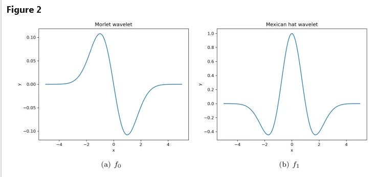
ENSO used a Descent optimization routine, while the AMO used the ADAM optimizer. AMO used a tanh activation function while ENSO fused a custom Gaussian wavelet, as the thought is that these are more effective for revealing Taylor's series expansion of a sinusoidal waveform. See also:

Uddin, Z., Ganga, S., Asthana, R. et al. Wavelets based physics informed neural networks to solve non-linear differential equations. Sci Rep 13, 2882 (2023). https://doi.org/10.1038/s41598-023-29806-

Twitter embedding may be broken due to the whims of Elon Musk.

Potentially could apply a rectified activation function here, such as relu or trelu, which may truncate negative excursions.

Marcus, S. L. Does an Intrinsic Source Generate a Shared Low-Frequency Signature in Earth’s Climate and Rotation Rate? Earth Interact.20, 1–14 (2015).

Mann, M. E., Steinman, B. A., Brouillette, D. J., & Miller, S. K. (2021). Multidecadal climate oscillations during the past millennium driven by volcanic forcing. Science, 371(6533), 1014-1019. In this paper, Mann and his co-authors presented evidence that the apparent oscillatory behavior of the AMO might be an artifact of the way the data is analyzed and that the true signal could be obscured by other external factors, such as volcanic eruptions and greenhouse gas emissions.