Machine Learning validates the ENSO model

The holy grail of climate science is being able to predict the next El Nino or La Nina several years in advance. The best we can do now is anticipate it by a few months. ML says hold my beer.

---

The observational record of El Nino and La Nina events are contained in temperature and atmospheric pressure time-series measurements collectively known as the El Nino Southern Oscillation (ENSO) climate indices. These are daunting to analyze as the climate cycles appear erratic. Predating these modern records are historical observations and proxies as described in the Encyclopedia of Paleoclimatology and Ancient Environments and elsewhere:

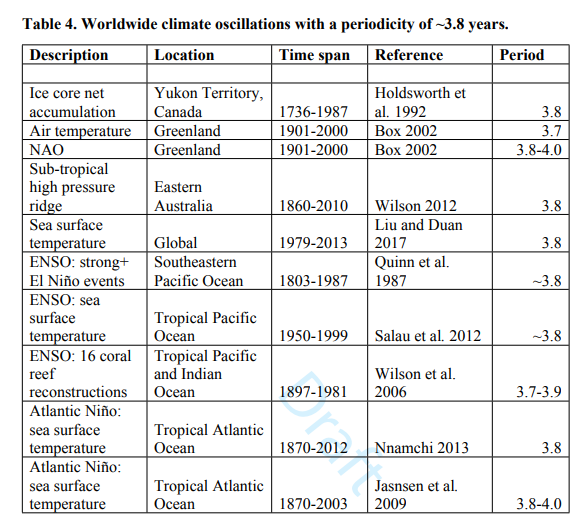
This period 3.8 years is key as it also describes the ecological cycles of wildlife populations such as lemmings and their prey, the arctic fox. An overlooked and still-uncited paper by Herb Archibald titled “Relating the 4-year lemming population cycle to a 3.8-year lunar cycle and ENSO” shows a linkage between ENSO cycles, phases of the moon, and how animals survive on the brink of existence. As a starting point, it’s an eye-opener and motivation for thinking outside the box. What I will describe next partially predates Herb’s publication, with the earlier foundational research documented in the text Mathematical Geonergy (Wiley/AGU, 2018).

First let me state that I’m not using AI to discover something new, as I already have a working geophysics-based model. In my view, the theoretical model comes first and the machine learning is only validating the canonical representation that was found from empirically fitting to the observations. So I am primarily using machine learning to validate what I already know, or at least believe may be correct. Thus, validation is only a means of further substantiating a model, as any proof is outside the realm of physics, and in this specific case that of geophysical fluid dynamics.

Premise

The basis of any ocean cycle model such as ENSO has to start with the unpredictable fluid dynamics of a body of water. Anyone that has tried to carry a shallow, wide bowl of soup across the room realizes how sensitive the fluid is to sudden changes in motion. That’s in fact how the cycles of ENSO are described: as an east-to-west-back-and-forth sloshing of the equatorial waters in the Pacific Ocean.

Yet, sloshing may sound counter-intuitive in that no one discusses huge variations of the ocean level on the coast or at coral atolls in the middle of the tropical Pacific. This sloshing in fact is primarily a subsurface effect. Consider that the subsurface thermocline is a metastable interface immersed within a low effective gravity environment. The action is all in the thermocline

¹

— slight density differences above and below the thermocline create a greatly reduced effective gravity which becomes sensitive to lunisolar forcing, just as with conventional ocean tides. This means that tidal forces can create much larger and more slowly evolving subsurface waves that reach to the surface. These can then drive multi-year global climate variations, via the El Nino events that occur when the subsurface thermocline sloshing reaches extremes relative to the surface.

The connection between the sloshing response and any causation can perhaps be calibrated by considering which sudden motions of the Earth’s own bowl of soup are driven by external forces. In fact, the moon and the sun are constantly speeding up and slowing down the Earth’s rotation rate, leading to precisely measurable changes in the length of day (LOD) measurement

²

. This is quite the eye-chart below but the graph shows the rate of change (1st derivative with respect to time) of LOD from 1962 onwards.

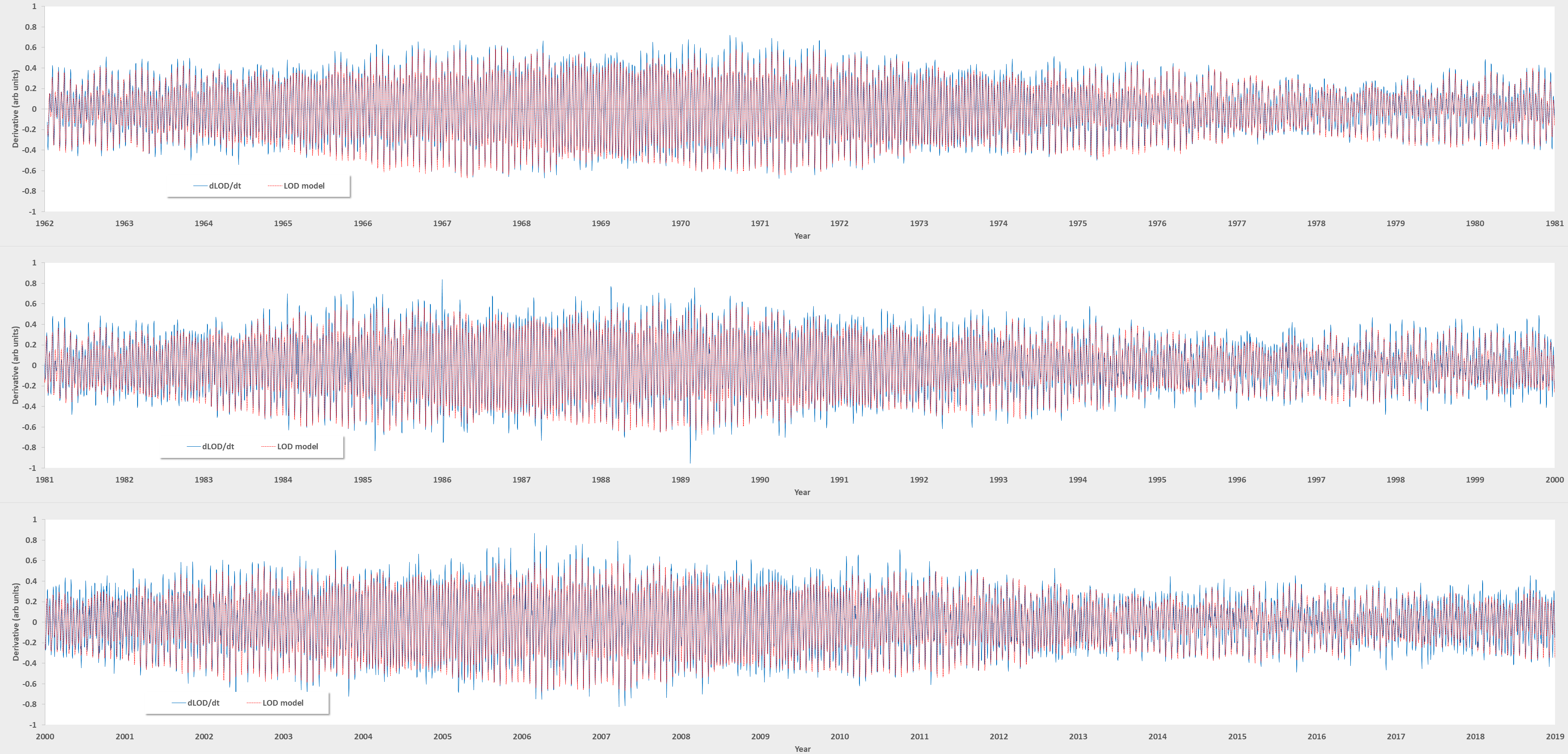
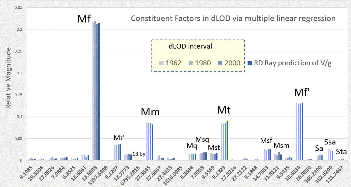
The main period is associated with the fortnightly 13.66 day Mf lunar tidal factor and the longer modulation with the 18.6 year period of lunar nodal declination, well known to create tidal extremes. The LOD' data shown above can be precisely fit to a Fourier series representation of all the primary tidal factors, thus allowing a model to extend back in time and also forward, analogous to conventional ocean tidal forecasting.

Clearly these LOD cycles don’t match to the average 3.8 year period of ENSO cycles

³

, yet this is not the only consideration when dealing with the characteristics of the ocean. Consider that semi-annually, impulse-like events corresponding to minimum density difference above and below the thermocline will occur. In dimictic freshwater lakes these dates of meta-stability link to fast turnover events of the water volume as an analogous semi-annual cycle. Along the equator, due to hemispherical symmetry, these would require to be aligned precisely at 6-month intervals.

The math expression for an alternating cycle of impulses (aka Kronecker delta functions) of equal and opposite directions, with equal time spacing, expressed as an infinite sum, multiplied by a function f(t) is:

\(\int_{-\infty}^{\infty} \left(\sum_{n=0}^{\infty} (-1)^n \delta(t-nT)\right) f(t) dt \)

When f(t) is calibrated to LOD' and T is set to 6 months, the convolution integration

⁴

over time reveals a choppy square-wave-like behavior with period ~3.8 years, and also modulated by an 18.6 year envelope. This is shown below as the upper panel, with Herb Archibald’s lunar cycle shown directly below it as a comparison — note that this is a true observable to the eye, as wildlife may also be tuned to this 3.8 year cycle either through visual cues of the moon phases or by climatic changes.

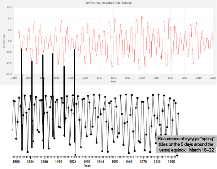
That’s the premise on how a combined lunisolar pattern could result in a roughly 3.8 year cycle. The detailed response leading to the erratic ENSO behavior lies in the fluid dynamics model.

Fluid Dynamics Model

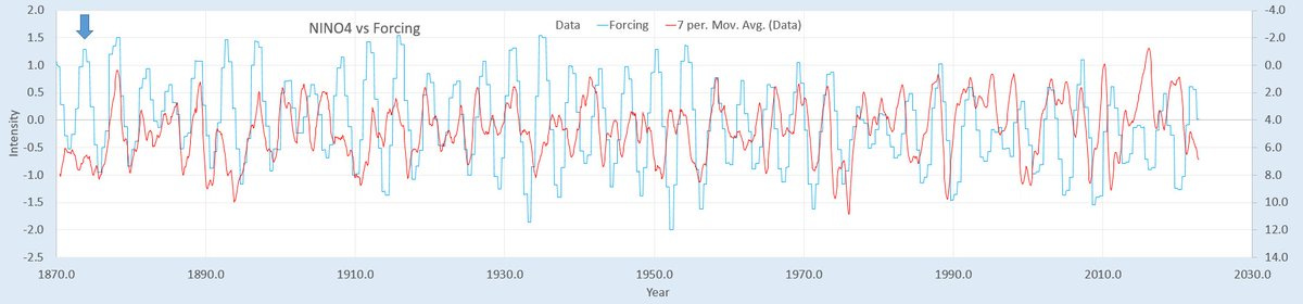
The characteristic one notices is that only with filtering of the ENSO time-series does the 3.8 year cycle vaguely reveal itself. As shown below, the RED line (in this case the NINO4 climate index) is still erratic in contrast to the more regular tidally forced cycle in BLUE.

So the educated guess is that something additional may be responsible for creating the erratic behavior. As a next premise, the fluid dynamics response to the lunar tidal forcing may be responsible for shaping the final response

⁵

. This is via a nonlinear effect in the solution of Laplace’s Tidal Equations (LTE), which is the standard formulation for solving fluid dynamics of a (relatively) shallow-water volume on a rotating planet with a Coriolis effect. In Chapter 12 of Mathematical Geoenergy

⁶

the details are fully described, but the general idea is that the forcing levels will get modulated by a sinusoidal multiplier which uses the tidal forcing level value as an input. I refer to this as a solution via LTE modulation.

This is not an intuitive way to think about wave dynamics, which is conventionally a temporally-derived sinusoidal response. But because the fluid dynamics occur essentially on a topologically constrained 1-D equatorial waveguide, and that the standing-wave modes of a finite ocean play into a separable spatial and temporal solution, evaluating such an atypical formulation is worth the effort

⁷

.

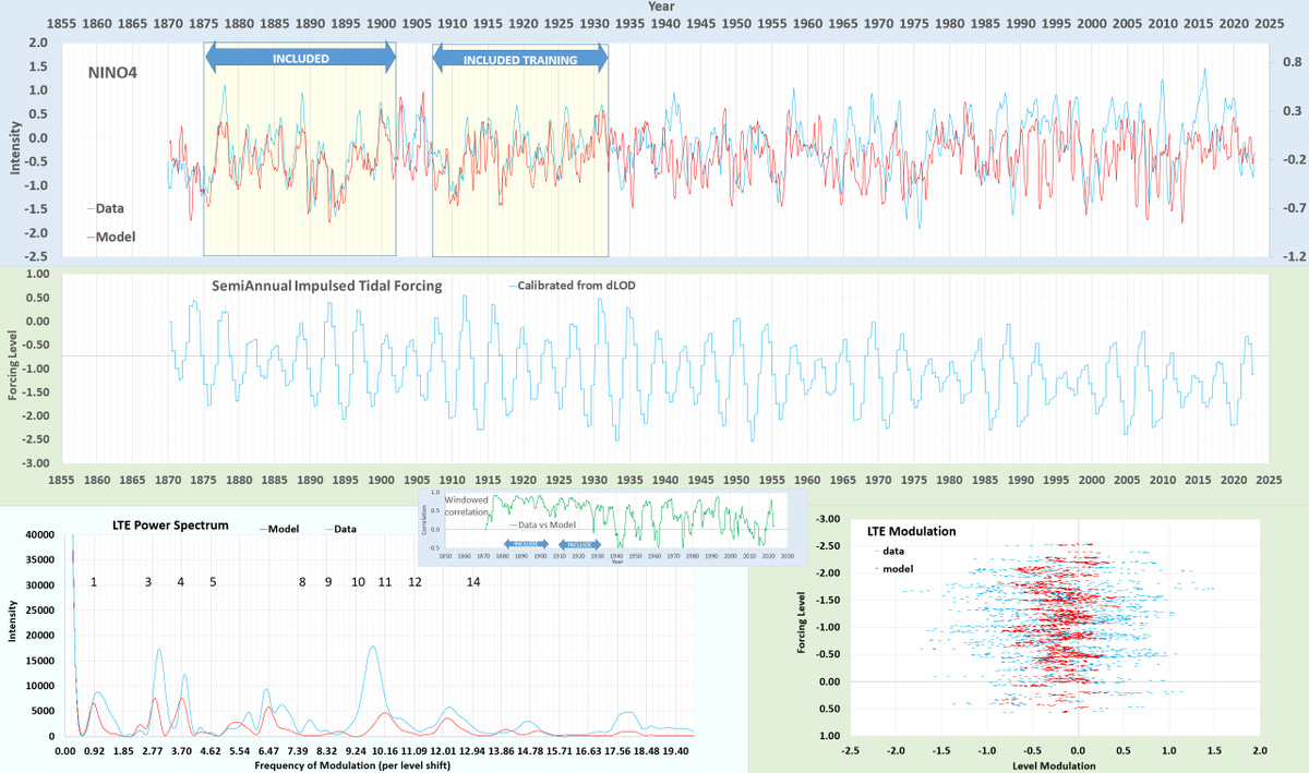
Because the solution is nonlinear and requires careful book-keeping of the tidal and modulation factors, I devised software for the empirical model fitting to the various climate indices. Applying an LTE modulation that features a fundamental sinusoidal factor and several harmonics

⁸

, an adequate fit to the NINO4 data can be obtained over the entire time span. More importantly, by training on a short interval, the model can be cross-validated on the rest of the interval. This is a guard against model over-fitting, see the shaded region in the upper panel below.

The caveat is that slight variations in the tidal factors are allowed as that benefits the randomized search from falling into local minimums of the loss function. The differences between a LOD calibrated forcing and one slightly adjusted is shown below.

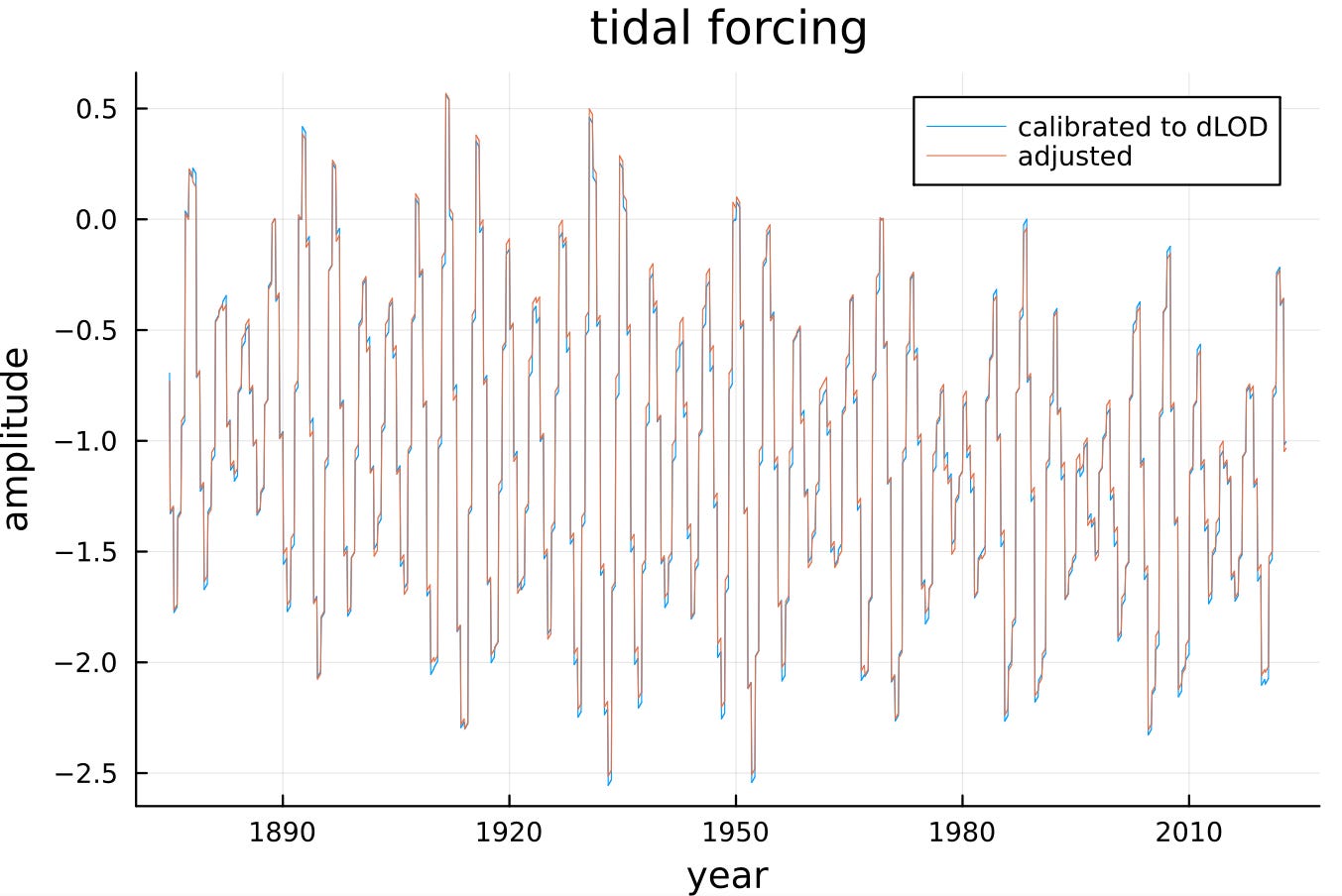
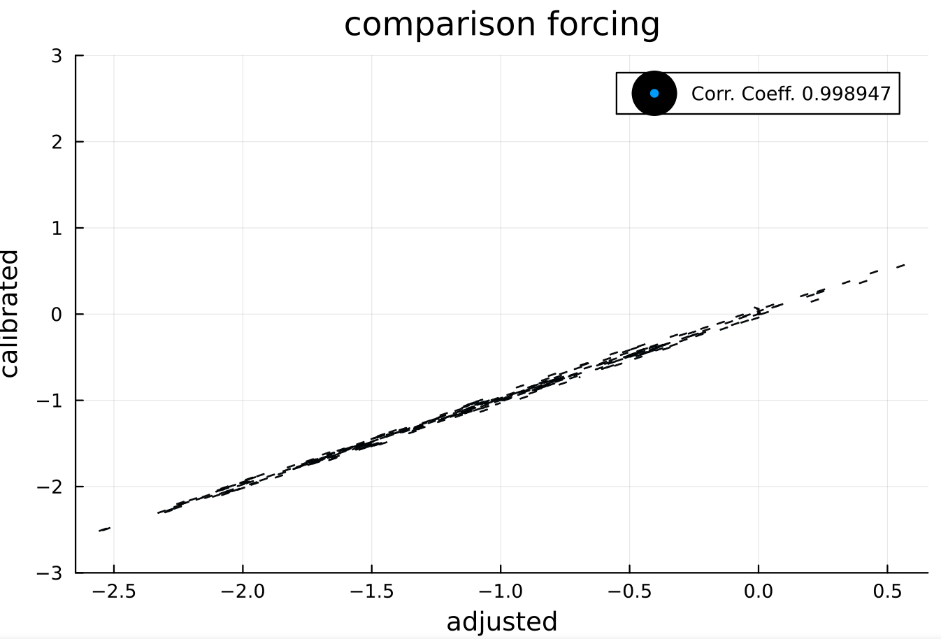
So this caveat is minor yet must be stated as part of the model training/fitting process. It may be that this slight variation is also more indicative of the actual tidal forcing.

This is not machine learning in the conventional sense in that it is simply searching a constrained parameter solution space instead of a wide-open unconstrained fully-connected neural network.

Machine Learning

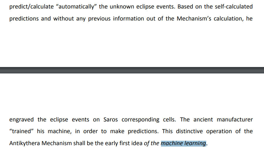
As it turns out, the earliest machine learning involved lunar and solar cycles, via the Antikythera Mechanism, recovered from an archaeological dig. By reverse engineering, researchers have found many intriguing cycles, including an Olympiad cycle of 4 years and sub-Metonic 3.8 (may this be the rational for the Olympics?)

Obviously we now have computers to do the machine learning instead of mechanical devices. I chose a neural network library called Flux written in the Julia language. Since the basis for why a NN works is often not well-formulated, the naive approach is to provide the tidal forcing described above as input (along with a normalized time axis) and the NINO4 as output to train against, with a mean-squared error as the loss function. All told about 50 lines of source code

⁹

.

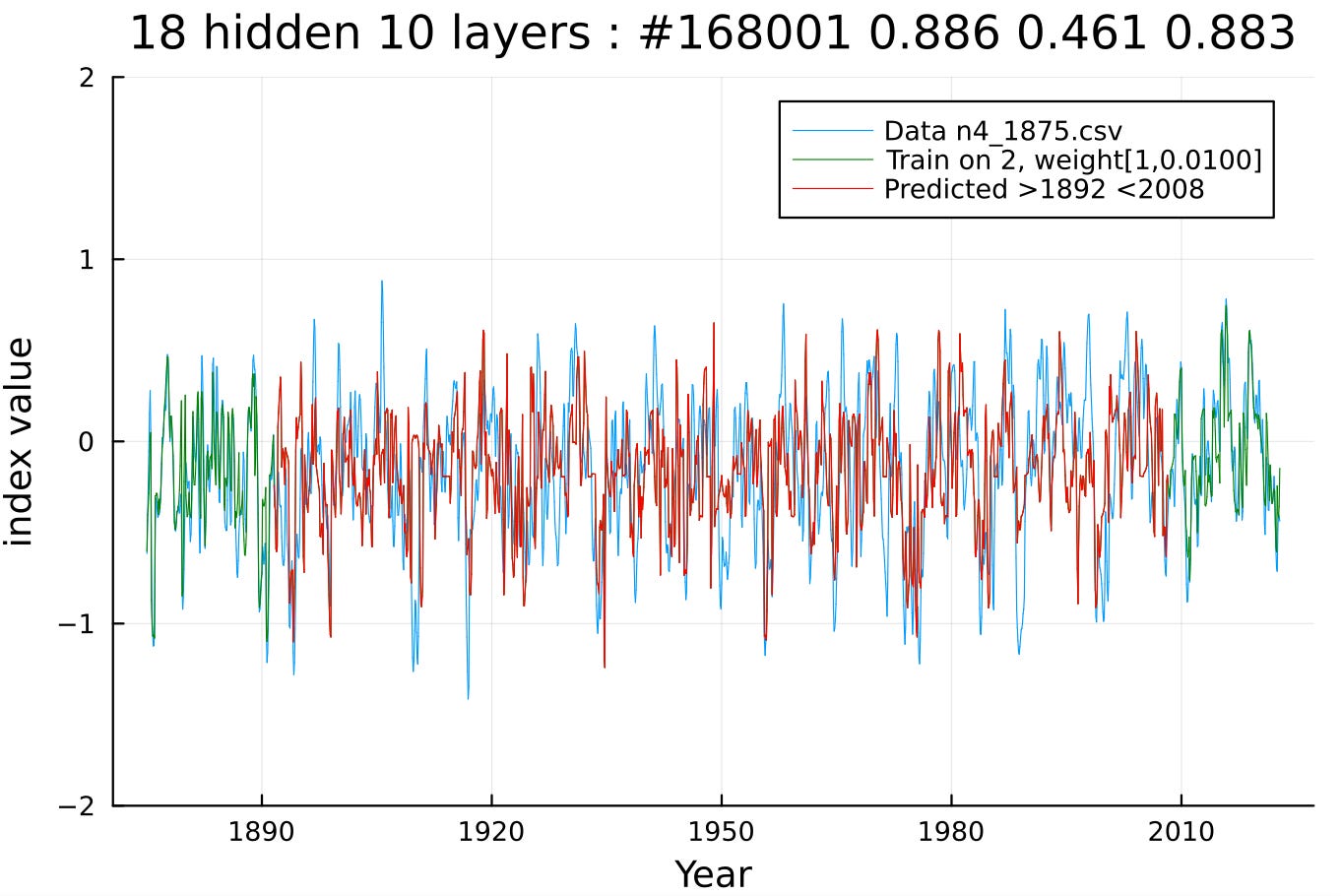
For training on NINO4, two intervals were chosen, near the beginning and near the end, with the ~100 year middle interval acting as a cross-validation test. The correlation coefficent in the middle “out-of-band” region of 0.192 is modest but significant as most runs will do equally well

¹⁰

:

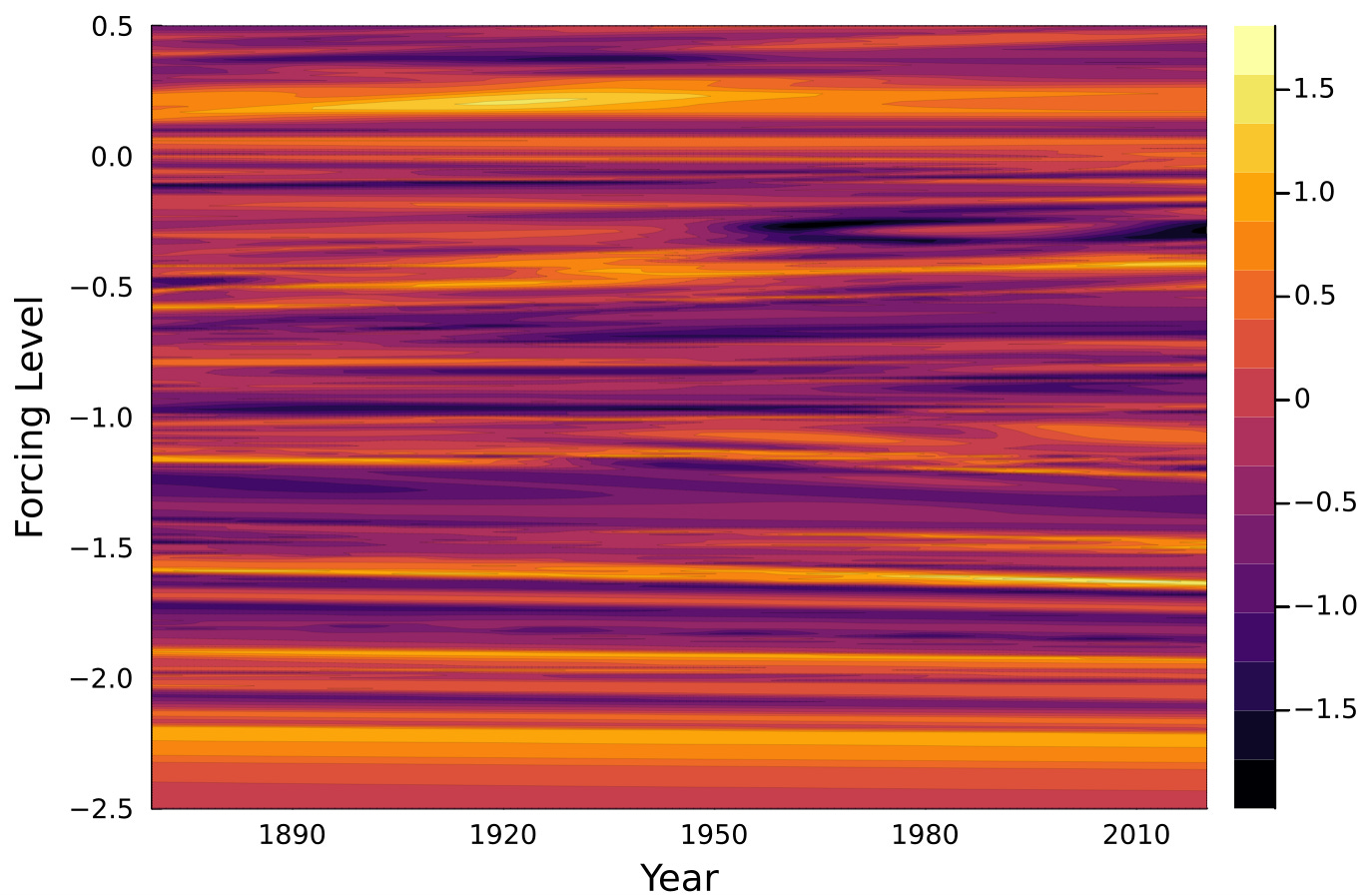
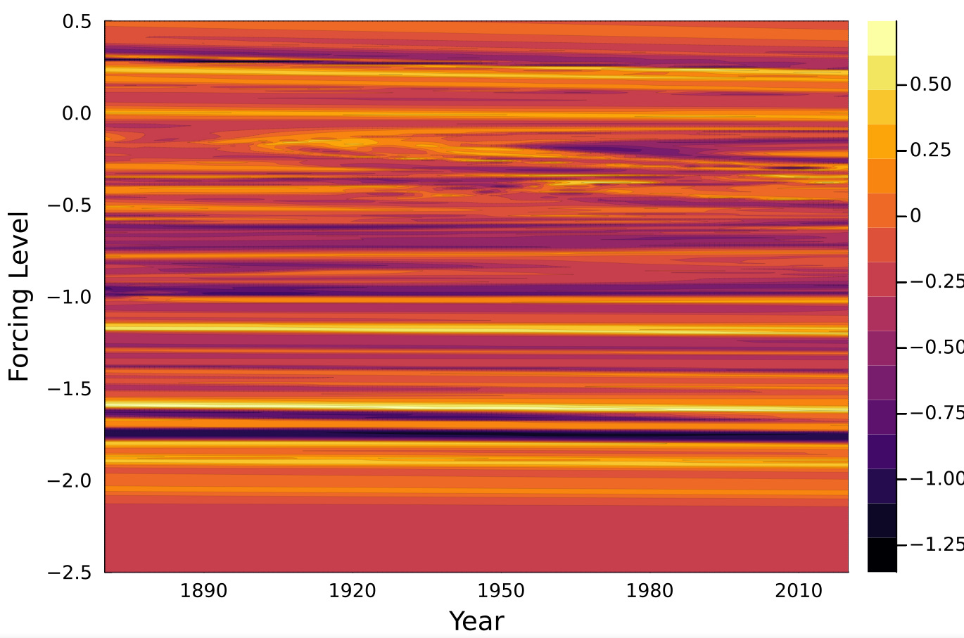
The time input is initially weighted low so that it doesn’t over-fit on that aspect, yet we can still look at how stationary the solution is across the entire interval. The following contour graph shows the modulation as a function of time, with the forcing level as the other NN input along the y-axis. Note that the modulation intensity (shaded by the scale on the right) is stationary with time, so that the modulation pre-1900 is the same as post-2000. Similar to reading a wavelet scalogram

¹¹

, the interpolated modulation remains primarily on horizontal striations, inferring a constant LTE modulation, and importantly cross-validating that as a mechanism - which we will further substantiate next.

What is likely occurring with the dense NN chain is that the layering is approximating a Taylor’s series of the sinusoidal modulation in the input to output mapping.

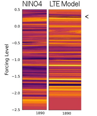
The check is to feed in the same forcing but this time use the LTE-modeled NINO4 as a training output instead of the actual NINO4 data set. The cross-validation correlation agreement improves markedly to 0.46, which is expected as these are pure sinusoidal harmonics being trained to — less complexity in terms of the simplicity bias known to occur in neural nets.

¹²

The stationarity across time is even more pronounced when training to the model, as the horizontal striations are flatter. This is expected as no time-dependency post tidal forcing was added to the LTE model modulation response. Whatever deviations are shown are likely a sign that the NN training is overfitting in that region.

Comparing the NN training of the actual data to the training of the LTE model side-by-side, one can see agreement in the forcing level positioning (see e.g. the level indicated by the < caret for an amplitude discrepancy), which indicates the trained NN chose similar sinusoidal LTE modulation to that chosen without the benefit of NN training.

Implications

One of the larger issues of neural networks is that they don’t always generalize well — in particular outside the training region. And if they do, it’s often difficult to reverse engineer the NN model to reveal the underlying physics. In this case of the LTE-based ENSO model, good news in both cases. The NN training generalizes well outside the training region, and reverse engineering is not necessary since the results agree with the canonical LTE-based model. The idea of adding time as an input could also be a valuable means of revealing time dependencies via NN scalagrams that show curved or sinusoidal striations.

And from a geophysical fluid dynamics standpoint, this provides a cross-validation of a model that may well solve a challenging climate variability problem — predicting what ENSO will do next.

Follow-on:

Machine Learning validates the AMO model

1. Zhao, S., Jin, F.-F., Long, X., & Cane, M. A. (2021). On the breakdown of ENSO's relationship with thermocline depth in the central-equatorial Pacific. Geophysical Research Letters, 48, e2020GL092335. https://doi.org/10.1029/2020GL092335 [Note: This paper notes that most regions of ENSO show that the subsurface thermocline matches the surface]

2. Ray, R. D., & Erofeeva, S. Y. (2014). Long‐period tidal variations in the length of day. Journal of Geophysical Research: Solid Earth, 119(2), 1498-1509

3. Lin, J., & Qian, T. (2019). Switch between el nino and la nina is caused by subsurface ocean waves likely driven by lunar tidal forcing. Scientific reports, 9(1), 1-10. [Note: this paper’s only failing is that it could not identify the periodicity of tidal forcing necessary to match the average ENSO period]

4. The integration is needed because a d/dt(LOD) was applied as an impulse and so the integration over time converts this to a LOD, so it’s essentially a conservation of momentum requirement.

5. Several years ago I had an online discussion with Nick Stokes, a grand-progeny of George Stokes of Navier-Stokes fame, who also happens to be fluid dynamic researcher. This provides insight from a practitioner with a different sense of intuition.

6. Pukite, P., Coyne, D., & Challou, D. (2018). Mathematical geoenergy: discovery, depletion, and renewal. John Wiley & Sons/American Geophysical Union.

7. Delplace, P., Marston, J. B., & Venaille, A. (2017). Topological origin of equatorial waves. Science, 358(6366), 1075-1077. [Note: This is a quite unconventional derivation applying concepts from topological insulators]

8. Harmonics are important in the solution as the bounding volume creates standing waves that fit into the basin in integer multiples of the spatial wavelength. The derivation of LTE sets up a linear relation between a spatial wavelength harmonic and an LTE modulation harmonic.

9. Source code under version control is available on GitHub. For this, snippets on the discussion area https://github.com/pukpr/GeoEnergyMath/discussions/23#discussioncomment-5576161

10. Depending on the complexity of the chain and the length of training interval, the fitting process can take just a few minutes. A speeded-up YouTube video of an early exploratory run for a lengthy training interval:

11. Prompt: What does flat horizontal shading of lines on a wavelet spectogram imply?
ChatGPT (v3.5): Flat horizontal shading of lines on a wavelet spectrogram generally indicates that there is no significant frequency or time variation in the signal at that particular time and frequency range.

12. Huh, M., Mobahi, H., Zhang, R., Cheung, B., Agrawal, P., & Isola, P. (2021). The low-rank simplicity bias in deep networks. arXiv preprint arXiv:2103.10427.